In this post, I will show you how to develop and assess a fake news classifier using Keras.

1. Acquire Training Data

We will first import the data set for this project. Here is the source of the data set. The following url contains the training data set.

import pandas as pd

train_url = "https://github.com/PhilChodrow/PIC16b/blob/master/datasets/fake_news_train.csv?raw=true"
train_data = pd.read_csv(train_url)
train_data.head()

	Unnamed: 0	title	text	fake
0	17366	Merkel: Strong result for Austria's FPO 'big c...	German Chancellor Angela Merkel said on Monday...	0
1	5634	Trump says Pence will lead voter fraud panel	WEST PALM BEACH, Fla.President Donald Trump sa...	0
2	17487	JUST IN: SUSPECTED LEAKER and “Close Confidant...	On December 5, 2017, Circa s Sara Carter warne...	1
3	12217	Thyssenkrupp has offered help to Argentina ove...	Germany s Thyssenkrupp, has offered assistance...	0
4	5535	Trump say appeals court decision on travel ban...	President Donald Trump on Thursday called the ...	0

Note that each row of the data corresponds to an article. The title column gives the title of the article, whereas the text column gives the full article text. The final column, fake, is 0 if the article is real news and 1 if the article is fake news.

2. Make a Dataset

Next, we will implement a function called make_dataset to clean our training data and prepare it for training. Here’s what the function looks like:

import numpy as np
import keras
from keras import layers
from keras import ops
import tensorflow as tf
from nltk.corpus import stopwords

def make_dataset(train_data):
  """ changes the text of training data to lowercase,
      removes stopwords from text and title, and returns
      a tf.data.Dataset with two inputs and one output """

  # converts text to lowercase
  train_data["text"] = train_data["text"].str.lower()

  # removes stopwords from title and text
  stop = stopwords.words('english') # loading english stop words
  train_data["title"] = train_data["title"].apply(
      lambda x: ' '.join([word for word in x.split() if word not in (stop)]))

  train_data["text"] = train_data["text"].apply(
      lambda x: ' '.join([word for word in x.split() if word not in (stop)]))

  dataset = tf.data.Dataset.from_tensor_slices((
      {"title": train_data["title"].values, # (title, text) as input
       "text": train_data["text"].values},
      train_data["fake"].values   # fake column as output
  ))

  # batching dataset (allows model to train on chunks rather than rows)
  dataset = dataset.batch(100)

  return dataset

dataset = make_dataset(train_data)
dataset

<_BatchDataset element_spec=({'title': TensorSpec(shape=(None,), dtype=tf.string, name=None), 'text': TensorSpec(shape=(None,), dtype=tf.string, name=None)}, TensorSpec(shape=(None,), dtype=tf.int64, name=None))>

Next, we will split 20% of our dataset to use for validation. Notice that we are using 45 batches for our validation data.

dataset = dataset.shuffle(buffer_size = len(dataset),
                       reshuffle_each_iteration = False)

train_size = int(0.8*len(dataset))
val_size = int(0.2*len(dataset))

train = dataset.take(train_size)
val   = dataset.skip(train_size).take(val_size)

len(train), len(val)

(180, 45)

We’ll now determine the base rate for our dataset by examining the labels on the training set. As we can see, the base rate is roughly 53%, which is what one might expect.

import pandas as pd

def calculate_base_rate(train_data):
    # Count the number of instances of each class (1 and 0)
    class_counts = train_data["fake"].value_counts()

    # Calculate the base rate by finding the max count divided by
    # total number of samples
    base_rate = class_counts.max() / class_counts.sum()

    return base_rate

# Calculate and print the base rate
base_rate = calculate_base_rate(train_data)
print("Base Rate:", base_rate)

Base Rate: 0.522963160942581

Finally, we will prepare a text vectorization layer for our tf model.

from tensorflow.keras.layers import TextVectorization
import re
import string

#preparing a text vectorization layer for tf model
size_vocabulary = 2000

def standardization(input_data):
    lowercase = tf.strings.lower(input_data)
    no_punctuation = tf.strings.regex_replace(lowercase,
                                  '[%s]' % re.escape(string.punctuation),'')
    return no_punctuation

title_vectorize_layer = TextVectorization(
    standardize=standardization,
    max_tokens=size_vocabulary, # only consider this many words
    output_mode='int',
    output_sequence_length=500)

title_vectorize_layer.adapt(train.map(lambda x, y: x["title"]))

text_vectorize_layer = TextVectorization(
    standardize=standardization,
    max_tokens=size_vocabulary, # only consider this many words
    output_mode='int',
    output_sequence_length=500)

text_vectorize_layer.adapt(train.map(lambda x, y: x["text"]))

3. Create Models

We will create three Keras model to offer a perspective the following question:

When detecting fake news, is it most effective to focus on only the title of the article, the full text of the article, or both?

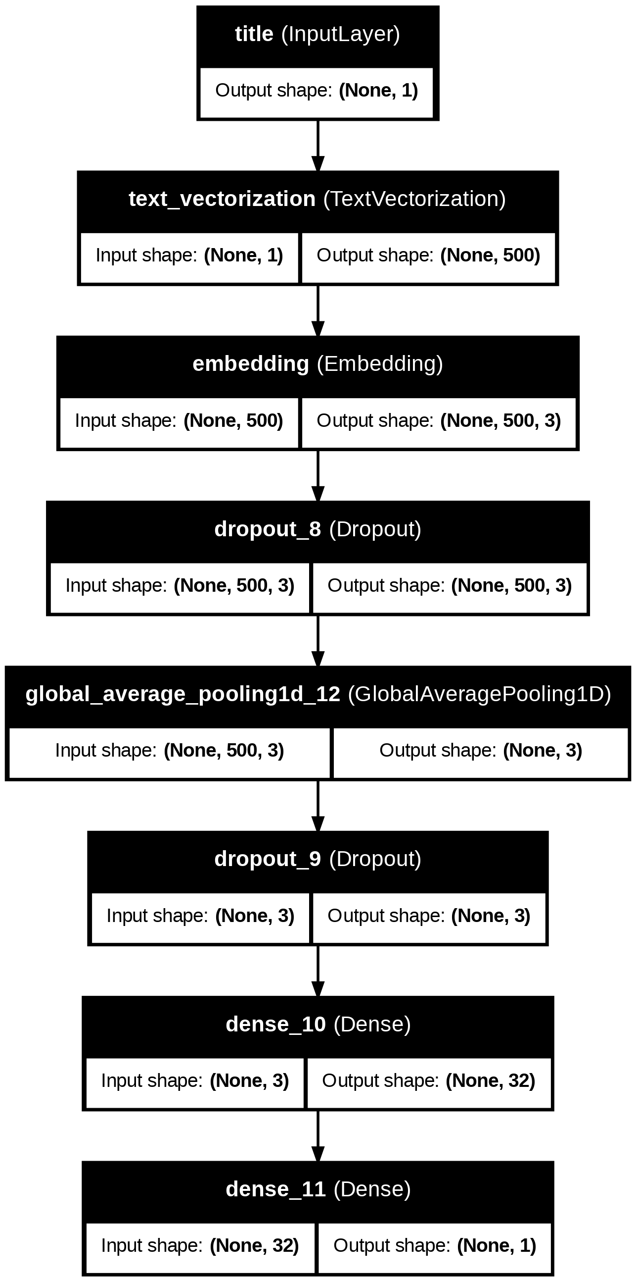
For the first model, we will use only the article title as input.

from tensorflow.keras.losses import BinaryCrossentropy

train_data = train.map(lambda x, y: x["title"])
title_vectorize_layer.adapt(train_data)

# input layer
title_input = keras.Input(shape=(1,), dtype="string", name="title")

# text processing layers
title_features = title_vectorize_layer(title_input)
title_features = layers.Embedding(size_vocabulary, 3, name="embedding")(title_features)
title_features = layers.Dropout(0.2)(title_features)
title_features = layers.GlobalAveragePooling1D()(title_features)
title_features = layers.Dropout(0.2)(title_features)
title_features = layers.Dense(32, activation='relu')(title_features)

# output layer
output = layers.Dense(1, activation='sigmoid')(title_features)


# model compilation (need to do this before training)
model1 = keras.Model(inputs=title_input, outputs=output)
model1.compile(optimizer='adam', loss='binary_crossentropy',
                    metrics=['accuracy'])

model1.summary()

Model: "functional_7"

┏━━━━━━━━━━━━━━━━━━━━━━━━━━━━━━━━━━━━━━┳━━━━━━━━━━━━━━━━━━━━━━━━━━━━━┳━━━━━━━━━━━━━━━━━┓
┃ Layer (type)                         ┃ Output Shape                ┃         Param # ┃
┡━━━━━━━━━━━━━━━━━━━━━━━━━━━━━━━━━━━━━━╇━━━━━━━━━━━━━━━━━━━━━━━━━━━━━╇━━━━━━━━━━━━━━━━━┩
│ title (InputLayer)                   │ (None, 1)                   │               0 │
├──────────────────────────────────────┼─────────────────────────────┼─────────────────┤
│ text_vectorization                   │ (None, 500)                 │               0 │
│ (TextVectorization)                  │                             │                 │
├──────────────────────────────────────┼─────────────────────────────┼─────────────────┤
│ embedding (Embedding)                │ (None, 500, 3)              │           6,000 │
├──────────────────────────────────────┼─────────────────────────────┼─────────────────┤
│ dropout_8 (Dropout)                  │ (None, 500, 3)              │               0 │
├──────────────────────────────────────┼─────────────────────────────┼─────────────────┤
│ global_average_pooling1d_12          │ (None, 3)                   │               0 │
│ (GlobalAveragePooling1D)             │                             │                 │
├──────────────────────────────────────┼─────────────────────────────┼─────────────────┤
│ dropout_9 (Dropout)                  │ (None, 3)                   │               0 │
├──────────────────────────────────────┼─────────────────────────────┼─────────────────┤
│ dense_10 (Dense)                     │ (None, 32)                  │             128 │
├──────────────────────────────────────┼─────────────────────────────┼─────────────────┤
│ dense_11 (Dense)                     │ (None, 1)                   │              33 │
└──────────────────────────────────────┴─────────────────────────────┴─────────────────┘

 Total params: 6,161 (24.07 KB)

 Trainable params: 6,161 (24.07 KB)

 Non-trainable params: 0 (0.00 B)

# to visualize the model

from keras import utils
utils.plot_model(model1, "output_filename.png",
                       show_shapes=True,
                       show_layer_names=True)

Now we train our model.

# implement callback for early stopping to prevent overfitting
callback = keras.callbacks.EarlyStopping(monitor='val_loss', patience=5)

# train model
history = model1.fit(train,
                    validation_data=val,
                    epochs = 50,
                    callbacks=[callback],
                    verbose = True)

Epoch 1/50
180/180 ━━━━━━━━━━━━━━━━━━━━ 8s 34ms/step - accuracy: 0.5263 - loss: 0.6890 - val_accuracy: 0.8038 - val_loss: 0.6404
Epoch 2/50
180/180 ━━━━━━━━━━━━━━━━━━━━ 9s 27ms/step - accuracy: 0.8175 - loss: 0.5799 - val_accuracy: 0.9451 - val_loss: 0.3571
Epoch 3/50
180/180 ━━━━━━━━━━━━━━━━━━━━ 6s 28ms/step - accuracy: 0.9034 - loss: 0.3341 - val_accuracy: 0.9218 - val_loss: 0.2310
Epoch 4/50
180/180 ━━━━━━━━━━━━━━━━━━━━ 4s 23ms/step - accuracy: 0.9200 - loss: 0.2399 - val_accuracy: 0.9253 - val_loss: 0.1896
Epoch 5/50
180/180 ━━━━━━━━━━━━━━━━━━━━ 4s 20ms/step - accuracy: 0.9359 - loss: 0.1982 - val_accuracy: 0.9187 - val_loss: 0.1785
Epoch 6/50
180/180 ━━━━━━━━━━━━━━━━━━━━ 8s 33ms/step - accuracy: 0.9346 - loss: 0.1861 - val_accuracy: 0.9178 - val_loss: 0.1721
Epoch 7/50
180/180 ━━━━━━━━━━━━━━━━━━━━ 8s 23ms/step - accuracy: 0.9419 - loss: 0.1732 - val_accuracy: 0.9304 - val_loss: 0.1544
Epoch 8/50
180/180 ━━━━━━━━━━━━━━━━━━━━ 5s 20ms/step - accuracy: 0.9456 - loss: 0.1605 - val_accuracy: 0.9420 - val_loss: 0.1401
Epoch 9/50
180/180 ━━━━━━━━━━━━━━━━━━━━ 5s 20ms/step - accuracy: 0.9461 - loss: 0.1510 - val_accuracy: 0.9318 - val_loss: 0.1473
Epoch 10/50
180/180 ━━━━━━━━━━━━━━━━━━━━ 6s 31ms/step - accuracy: 0.9489 - loss: 0.1432 - val_accuracy: 0.9484 - val_loss: 0.1268
Epoch 11/50
180/180 ━━━━━━━━━━━━━━━━━━━━ 4s 22ms/step - accuracy: 0.9529 - loss: 0.1387 - val_accuracy: 0.9518 - val_loss: 0.1197
Epoch 12/50
180/180 ━━━━━━━━━━━━━━━━━━━━ 5s 20ms/step - accuracy: 0.9566 - loss: 0.1315 - val_accuracy: 0.9736 - val_loss: 0.1140
Epoch 13/50
180/180 ━━━━━━━━━━━━━━━━━━━━ 7s 32ms/step - accuracy: 0.9585 - loss: 0.1236 - val_accuracy: 0.9498 - val_loss: 0.1200
Epoch 14/50
180/180 ━━━━━━━━━━━━━━━━━━━━ 4s 20ms/step - accuracy: 0.9564 - loss: 0.1222 - val_accuracy: 0.9529 - val_loss: 0.1128
Epoch 15/50
180/180 ━━━━━━━━━━━━━━━━━━━━ 8s 34ms/step - accuracy: 0.9593 - loss: 0.1132 - val_accuracy: 0.9458 - val_loss: 0.1232
Epoch 16/50
180/180 ━━━━━━━━━━━━━━━━━━━━ 4s 21ms/step - accuracy: 0.9578 - loss: 0.1207 - val_accuracy: 0.9504 - val_loss: 0.1169
Epoch 17/50
180/180 ━━━━━━━━━━━━━━━━━━━━ 4s 20ms/step - accuracy: 0.9614 - loss: 0.1091 - val_accuracy: 0.9544 - val_loss: 0.1068
Epoch 18/50
180/180 ━━━━━━━━━━━━━━━━━━━━ 6s 28ms/step - accuracy: 0.9612 - loss: 0.1090 - val_accuracy: 0.9549 - val_loss: 0.1049
Epoch 19/50
180/180 ━━━━━━━━━━━━━━━━━━━━ 4s 21ms/step - accuracy: 0.9593 - loss: 0.1082 - val_accuracy: 0.9564 - val_loss: 0.1032
Epoch 20/50
180/180 ━━━━━━━━━━━━━━━━━━━━ 5s 20ms/step - accuracy: 0.9630 - loss: 0.1005 - val_accuracy: 0.9551 - val_loss: 0.1044
Epoch 21/50
180/180 ━━━━━━━━━━━━━━━━━━━━ 7s 32ms/step - accuracy: 0.9616 - loss: 0.1012 - val_accuracy: 0.9540 - val_loss: 0.1082
Epoch 22/50
180/180 ━━━━━━━━━━━━━━━━━━━━ 4s 21ms/step - accuracy: 0.9661 - loss: 0.0966 - val_accuracy: 0.9549 - val_loss: 0.1027
Epoch 23/50
180/180 ━━━━━━━━━━━━━━━━━━━━ 4s 23ms/step - accuracy: 0.9638 - loss: 0.0972 - val_accuracy: 0.9544 - val_loss: 0.1038
Epoch 24/50
180/180 ━━━━━━━━━━━━━━━━━━━━ 5s 25ms/step - accuracy: 0.9652 - loss: 0.0931 - val_accuracy: 0.9780 - val_loss: 0.0962
Epoch 25/50
180/180 ━━━━━━━━━━━━━━━━━━━━ 6s 28ms/step - accuracy: 0.9687 - loss: 0.0883 - val_accuracy: 0.9776 - val_loss: 0.0956
Epoch 26/50
180/180 ━━━━━━━━━━━━━━━━━━━━ 11s 32ms/step - accuracy: 0.9664 - loss: 0.0908 - val_accuracy: 0.9553 - val_loss: 0.1004
Epoch 27/50
180/180 ━━━━━━━━━━━━━━━━━━━━ 5s 29ms/step - accuracy: 0.9662 - loss: 0.0882 - val_accuracy: 0.9769 - val_loss: 0.0926
Epoch 28/50
180/180 ━━━━━━━━━━━━━━━━━━━━ 9s 21ms/step - accuracy: 0.9686 - loss: 0.0857 - val_accuracy: 0.9776 - val_loss: 0.0880
Epoch 29/50
180/180 ━━━━━━━━━━━━━━━━━━━━ 5s 27ms/step - accuracy: 0.9705 - loss: 0.0806 - val_accuracy: 0.9782 - val_loss: 0.0901
Epoch 30/50
180/180 ━━━━━━━━━━━━━━━━━━━━ 4s 21ms/step - accuracy: 0.9715 - loss: 0.0789 - val_accuracy: 0.9789 - val_loss: 0.0889
Epoch 31/50
180/180 ━━━━━━━━━━━━━━━━━━━━ 4s 20ms/step - accuracy: 0.9700 - loss: 0.0803 - val_accuracy: 0.9778 - val_loss: 0.0918
Epoch 32/50
180/180 ━━━━━━━━━━━━━━━━━━━━ 4s 23ms/step - accuracy: 0.9745 - loss: 0.0742 - val_accuracy: 0.9784 - val_loss: 0.0868
Epoch 33/50
180/180 ━━━━━━━━━━━━━━━━━━━━ 5s 21ms/step - accuracy: 0.9715 - loss: 0.0752 - val_accuracy: 0.9756 - val_loss: 0.0914
Epoch 34/50
180/180 ━━━━━━━━━━━━━━━━━━━━ 4s 20ms/step - accuracy: 0.9698 - loss: 0.0771 - val_accuracy: 0.9780 - val_loss: 0.0927
Epoch 35/50
180/180 ━━━━━━━━━━━━━━━━━━━━ 7s 31ms/step - accuracy: 0.9681 - loss: 0.0814 - val_accuracy: 0.9567 - val_loss: 0.0978
Epoch 36/50
180/180 ━━━━━━━━━━━━━━━━━━━━ 4s 20ms/step - accuracy: 0.9712 - loss: 0.0743 - val_accuracy: 0.9784 - val_loss: 0.0915
Epoch 37/50
180/180 ━━━━━━━━━━━━━━━━━━━━ 4s 20ms/step - accuracy: 0.9684 - loss: 0.0834 - val_accuracy: 0.9780 - val_loss: 0.0843
Epoch 38/50
180/180 ━━━━━━━━━━━━━━━━━━━━ 5s 29ms/step - accuracy: 0.9756 - loss: 0.0672 - val_accuracy: 0.9769 - val_loss: 0.0861
Epoch 39/50
180/180 ━━━━━━━━━━━━━━━━━━━━ 9s 20ms/step - accuracy: 0.9720 - loss: 0.0735 - val_accuracy: 0.9767 - val_loss: 0.0893
Epoch 40/50
180/180 ━━━━━━━━━━━━━━━━━━━━ 5s 29ms/step - accuracy: 0.9740 - loss: 0.0682 - val_accuracy: 0.9778 - val_loss: 0.0846
Epoch 41/50
180/180 ━━━━━━━━━━━━━━━━━━━━ 9s 20ms/step - accuracy: 0.9758 - loss: 0.0667 - val_accuracy: 0.9767 - val_loss: 0.0945
Epoch 42/50
180/180 ━━━━━━━━━━━━━━━━━━━━ 7s 29ms/step - accuracy: 0.9747 - loss: 0.0656 - val_accuracy: 0.9780 - val_loss: 0.0913

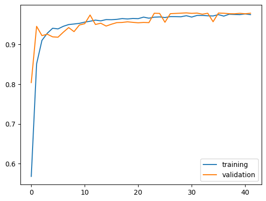
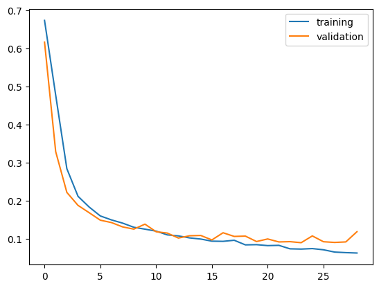
from matplotlib import pyplot as plt
plt.plot(history.history["accuracy"],label='training')
plt.plot(history.history["val_accuracy"],label='validation')
plt.legend()

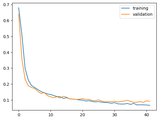
plt.plot(history.history["loss"],label='training')
plt.plot(history.history["val_loss"],label='validation')
plt.legend()

It appears that model1’s accuracy ranges between 96% and 97.5%.

For the second model, we will use only the article text as input. Once again, we’ll compile and then train the model.

train_texts = train.map(lambda x, y: x['text'])
text_vectorize_layer.adapt(train_texts)

# input Layer
text_input = keras.Input(shape=(1,), dtype="string", name="text")

# text processing layers
text_features = text_vectorize_layer(text_input)
text_features = layers.Embedding(size_vocabulary, 3, name="embedding")(text_features)
text_features = layers.Dropout(0.2)(text_features)
text_features = layers.GlobalAveragePooling1D()(text_features)
text_features = layers.Dropout(0.2)(text_features)
text_features = layers.Dense(32, activation='relu')(text_features)

# output layer
output = layers.Dense(1, activation='sigmoid')(text_features)

# Model Compilation
model2 = keras.Model(inputs=text_input, outputs=output)
model2.compile(optimizer='adam', loss='binary_crossentropy',
                    metrics=['accuracy'])
model2.summary()

Model: "functional_8"

┏━━━━━━━━━━━━━━━━━━━━━━━━━━━━━━━━━━━━━━┳━━━━━━━━━━━━━━━━━━━━━━━━━━━━━┳━━━━━━━━━━━━━━━━━┓
┃ Layer (type)                         ┃ Output Shape                ┃         Param # ┃
┡━━━━━━━━━━━━━━━━━━━━━━━━━━━━━━━━━━━━━━╇━━━━━━━━━━━━━━━━━━━━━━━━━━━━━╇━━━━━━━━━━━━━━━━━┩
│ text (InputLayer)                    │ (None, 1)                   │               0 │
├──────────────────────────────────────┼─────────────────────────────┼─────────────────┤
│ text_vectorization_1                 │ (None, 500)                 │               0 │
│ (TextVectorization)                  │                             │                 │
├──────────────────────────────────────┼─────────────────────────────┼─────────────────┤
│ embedding (Embedding)                │ (None, 500, 3)              │           6,000 │
├──────────────────────────────────────┼─────────────────────────────┼─────────────────┤
│ dropout_10 (Dropout)                 │ (None, 500, 3)              │               0 │
├──────────────────────────────────────┼─────────────────────────────┼─────────────────┤
│ global_average_pooling1d_13          │ (None, 3)                   │               0 │
│ (GlobalAveragePooling1D)             │                             │                 │
├──────────────────────────────────────┼─────────────────────────────┼─────────────────┤
│ dropout_11 (Dropout)                 │ (None, 3)                   │               0 │
├──────────────────────────────────────┼─────────────────────────────┼─────────────────┤
│ dense_12 (Dense)                     │ (None, 32)                  │             128 │
├──────────────────────────────────────┼─────────────────────────────┼─────────────────┤
│ dense_13 (Dense)                     │ (None, 1)                   │              33 │
└──────────────────────────────────────┴─────────────────────────────┴─────────────────┘

 Total params: 6,161 (24.07 KB)

 Trainable params: 6,161 (24.07 KB)

 Non-trainable params: 0 (0.00 B)

# to visualize the model

utils.plot_model(model2, "output_filename.png",
                       show_shapes=True,
                       show_layer_names=True)

# implement callback for early stopping to prevent overfitting
callback = keras.callbacks.EarlyStopping(monitor='val_loss', patience=5)

# train model
history = model2.fit(train,
                    validation_data=val,
                    epochs = 50,
                    callbacks=[callback],
                    verbose = True)

Epoch 1/50
180/180 ━━━━━━━━━━━━━━━━━━━━ 6s 21ms/step - accuracy: 0.5335 - loss: 0.6873 - val_accuracy: 0.8627 - val_loss: 0.6162
Epoch 2/50
180/180 ━━━━━━━━━━━━━━━━━━━━ 9s 42ms/step - accuracy: 0.8523 - loss: 0.5490 - val_accuracy: 0.9489 - val_loss: 0.3287
Epoch 3/50
180/180 ━━━━━━━━━━━━━━━━━━━━ 5s 24ms/step - accuracy: 0.9127 - loss: 0.3132 - val_accuracy: 0.9229 - val_loss: 0.2216
Epoch 4/50
180/180 ━━━━━━━━━━━━━━━━━━━━ 4s 20ms/step - accuracy: 0.9291 - loss: 0.2258 - val_accuracy: 0.9189 - val_loss: 0.1876
Epoch 5/50
180/180 ━━━━━━━━━━━━━━━━━━━━ 6s 26ms/step - accuracy: 0.9337 - loss: 0.1943 - val_accuracy: 0.9260 - val_loss: 0.1683
Epoch 6/50
180/180 ━━━━━━━━━━━━━━━━━━━━ 4s 20ms/step - accuracy: 0.9443 - loss: 0.1668 - val_accuracy: 0.9358 - val_loss: 0.1487
Epoch 7/50
180/180 ━━━━━━━━━━━━━━━━━━━━ 6s 23ms/step - accuracy: 0.9461 - loss: 0.1542 - val_accuracy: 0.9356 - val_loss: 0.1424
Epoch 8/50
180/180 ━━━━━━━━━━━━━━━━━━━━ 5s 21ms/step - accuracy: 0.9473 - loss: 0.1461 - val_accuracy: 0.9447 - val_loss: 0.1310
Epoch 9/50
180/180 ━━━━━━━━━━━━━━━━━━━━ 4s 20ms/step - accuracy: 0.9509 - loss: 0.1354 - val_accuracy: 0.9478 - val_loss: 0.1252
Epoch 10/50
180/180 ━━━━━━━━━━━━━━━━━━━━ 6s 27ms/step - accuracy: 0.9534 - loss: 0.1321 - val_accuracy: 0.9371 - val_loss: 0.1382
Epoch 11/50
180/180 ━━━━━━━━━━━━━━━━━━━━ 4s 20ms/step - accuracy: 0.9532 - loss: 0.1277 - val_accuracy: 0.9498 - val_loss: 0.1184
Epoch 12/50
180/180 ━━━━━━━━━━━━━━━━━━━━ 4s 20ms/step - accuracy: 0.9564 - loss: 0.1149 - val_accuracy: 0.9513 - val_loss: 0.1149
Epoch 13/50
180/180 ━━━━━━━━━━━━━━━━━━━━ 4s 23ms/step - accuracy: 0.9591 - loss: 0.1120 - val_accuracy: 0.9609 - val_loss: 0.1018
Epoch 14/50
180/180 ━━━━━━━━━━━━━━━━━━━━ 5s 21ms/step - accuracy: 0.9618 - loss: 0.1044 - val_accuracy: 0.9542 - val_loss: 0.1078
Epoch 15/50
180/180 ━━━━━━━━━━━━━━━━━━━━ 4s 20ms/step - accuracy: 0.9639 - loss: 0.1021 - val_accuracy: 0.9529 - val_loss: 0.1085
Epoch 16/50
180/180 ━━━━━━━━━━━━━━━━━━━━ 5s 26ms/step - accuracy: 0.9631 - loss: 0.0975 - val_accuracy: 0.9609 - val_loss: 0.0968
Epoch 17/50
180/180 ━━━━━━━━━━━━━━━━━━━━ 4s 21ms/step - accuracy: 0.9620 - loss: 0.0958 - val_accuracy: 0.9458 - val_loss: 0.1157
Epoch 18/50
180/180 ━━━━━━━━━━━━━━━━━━━━ 4s 20ms/step - accuracy: 0.9605 - loss: 0.1071 - val_accuracy: 0.9542 - val_loss: 0.1060
Epoch 19/50
180/180 ━━━━━━━━━━━━━━━━━━━━ 6s 27ms/step - accuracy: 0.9673 - loss: 0.0880 - val_accuracy: 0.9533 - val_loss: 0.1069
Epoch 20/50
180/180 ━━━━━━━━━━━━━━━━━━━━ 4s 20ms/step - accuracy: 0.9646 - loss: 0.0891 - val_accuracy: 0.9598 - val_loss: 0.0926
Epoch 21/50
180/180 ━━━━━━━━━━━━━━━━━━━━ 5s 20ms/step - accuracy: 0.9667 - loss: 0.0844 - val_accuracy: 0.9580 - val_loss: 0.0994
Epoch 22/50
180/180 ━━━━━━━━━━━━━━━━━━━━ 7s 29ms/step - accuracy: 0.9658 - loss: 0.0888 - val_accuracy: 0.9602 - val_loss: 0.0916
Epoch 23/50
180/180 ━━━━━━━━━━━━━━━━━━━━ 9s 20ms/step - accuracy: 0.9685 - loss: 0.0788 - val_accuracy: 0.9600 - val_loss: 0.0923
Epoch 24/50
180/180 ━━━━━━━━━━━━━━━━━━━━ 6s 25ms/step - accuracy: 0.9702 - loss: 0.0755 - val_accuracy: 0.9633 - val_loss: 0.0896
Epoch 25/50
180/180 ━━━━━━━━━━━━━━━━━━━━ 4s 20ms/step - accuracy: 0.9684 - loss: 0.0788 - val_accuracy: 0.9531 - val_loss: 0.1074
Epoch 26/50
180/180 ━━━━━━━━━━━━━━━━━━━━ 6s 26ms/step - accuracy: 0.9712 - loss: 0.0748 - val_accuracy: 0.9593 - val_loss: 0.0921
Epoch 27/50
180/180 ━━━━━━━━━━━━━━━━━━━━ 4s 20ms/step - accuracy: 0.9726 - loss: 0.0703 - val_accuracy: 0.9607 - val_loss: 0.0903
Epoch 28/50
180/180 ━━━━━━━━━━━━━━━━━━━━ 5s 20ms/step - accuracy: 0.9743 - loss: 0.0654 - val_accuracy: 0.9596 - val_loss: 0.0916
Epoch 29/50
180/180 ━━━━━━━━━━━━━━━━━━━━ 5s 28ms/step - accuracy: 0.9755 - loss: 0.0656 - val_accuracy: 0.9482 - val_loss: 0.1184

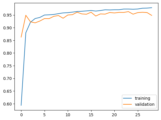
plt.plot(history.history["accuracy"],label='training')
plt.plot(history.history["val_accuracy"],label='validation')
plt.legend()

plt.plot(history.history["loss"],label='training')
plt.plot(history.history["val_loss"],label='validation')
plt.legend()

It appears that model2’s accuracy ranges between 96.5% and 97.5%, which is a slight improvement compared to model1.

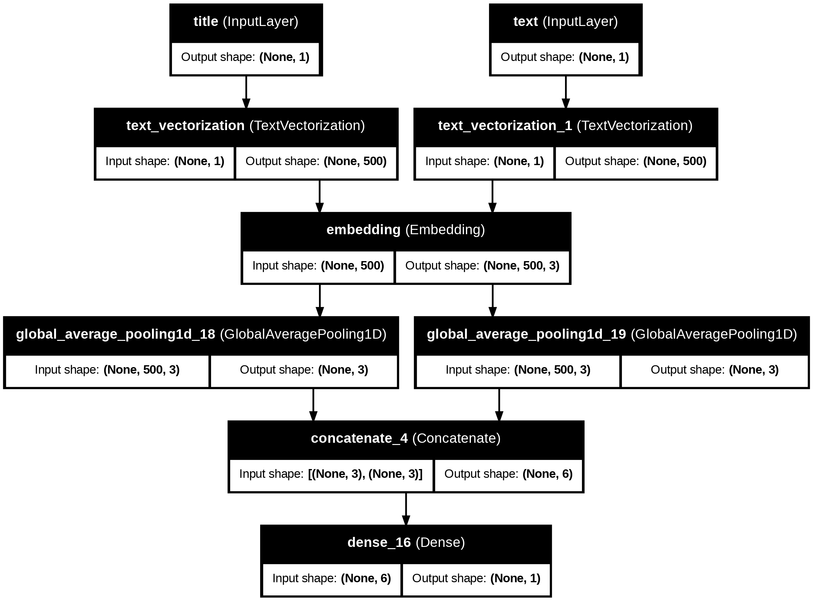
For the third model, we will use both the article title and the article text as input.

from tensorflow.keras.layers import TextVectorization, Embedding, Dropout, GlobalAveragePooling1D, Dense, Input, concatenate

train_data = train.map(lambda x, y: (x["title"], x["text"]))
train_titles, train_texts = zip(*train_data)

shared_embedding = Embedding(size_vocabulary, 3, name = "embedding")

title_input = Input(shape=(1,), dtype=tf.string, name="title")
title_vectorized = title_vectorize_layer(title_input)
title_embedded = shared_embedding(title_vectorized)
title_processed = GlobalAveragePooling1D()(title_embedded)

text_input = Input(shape=(1,), dtype=tf.string, name="text")
text_vectorized = text_vectorize_layer(text_input)
text_embedded = shared_embedding(text_vectorized)
text_processed = GlobalAveragePooling1D()(text_embedded)

combined_features = concatenate([title_processed, text_processed])
output = Dense(1, activation='sigmoid')(combined_features)

model3 = keras.Model(inputs=[title_input, text_input], outputs=output)
model3.compile(optimizer='adam', loss='binary_crossentropy',
                    metrics=['accuracy'])

model3.summary()

Model: "functional_11"

┏━━━━━━━━━━━━━━━━━━━━━━━━━━━┳━━━━━━━━━━━━━━━━━━━━━━━━┳━━━━━━━━━━━━━━━━┳━━━━━━━━━━━━━━━━━━━━━━━━┓
┃ Layer (type)              ┃ Output Shape           ┃        Param # ┃ Connected to           ┃
┡━━━━━━━━━━━━━━━━━━━━━━━━━━━╇━━━━━━━━━━━━━━━━━━━━━━━━╇━━━━━━━━━━━━━━━━╇━━━━━━━━━━━━━━━━━━━━━━━━┩
│ title (InputLayer)        │ (None, 1)              │              0 │ -                      │
├───────────────────────────┼────────────────────────┼────────────────┼────────────────────────┤
│ text (InputLayer)         │ (None, 1)              │              0 │ -                      │
├───────────────────────────┼────────────────────────┼────────────────┼────────────────────────┤
│ text_vectorization        │ (None, 500)            │              0 │ title[0][0]            │
│ (TextVectorization)       │                        │                │                        │
├───────────────────────────┼────────────────────────┼────────────────┼────────────────────────┤
│ text_vectorization_1      │ (None, 500)            │              0 │ text[0][0]             │
│ (TextVectorization)       │                        │                │                        │
├───────────────────────────┼────────────────────────┼────────────────┼────────────────────────┤
│ embedding (Embedding)     │ (None, 500, 3)         │          6,000 │ text_vectorization[7]… │
│                           │                        │                │ text_vectorization_1[… │
├───────────────────────────┼────────────────────────┼────────────────┼────────────────────────┤
│ global_average_pooling1d… │ (None, 3)              │              0 │ embedding[0][0]        │
│ (GlobalAveragePooling1D)  │                        │                │                        │
├───────────────────────────┼────────────────────────┼────────────────┼────────────────────────┤
│ global_average_pooling1d… │ (None, 3)              │              0 │ embedding[1][0]        │
│ (GlobalAveragePooling1D)  │                        │                │                        │
├───────────────────────────┼────────────────────────┼────────────────┼────────────────────────┤
│ concatenate_4             │ (None, 6)              │              0 │ global_average_poolin… │
│ (Concatenate)             │                        │                │ global_average_poolin… │
├───────────────────────────┼────────────────────────┼────────────────┼────────────────────────┤
│ dense_16 (Dense)          │ (None, 1)              │              7 │ concatenate_4[0][0]    │
└───────────────────────────┴────────────────────────┴────────────────┴────────────────────────┘

 Total params: 6,007 (23.46 KB)

 Trainable params: 6,007 (23.46 KB)

 Non-trainable params: 0 (0.00 B)

utils.plot_model(model3, "output_filename.png",
                       show_shapes=True,
                       show_layer_names=True)

# implement callback for early stopping to prevent overfitting
callback = keras.callbacks.EarlyStopping(monitor='val_loss', patience=5)

# train model
history = model3.fit(train,
                    validation_data=val,
                    epochs = 50,
                    callbacks=[callback],
                    verbose = True)

Epoch 1/50
180/180 ━━━━━━━━━━━━━━━━━━━━ 7s 30ms/step - accuracy: 0.5798 - loss: 0.6851 - val_accuracy: 0.6607 - val_loss: 0.6560
Epoch 2/50
180/180 ━━━━━━━━━━━━━━━━━━━━ 5s 26ms/step - accuracy: 0.6959 - loss: 0.6448 - val_accuracy: 0.7358 - val_loss: 0.6053
Epoch 3/50
180/180 ━━━━━━━━━━━━━━━━━━━━ 4s 20ms/step - accuracy: 0.7639 - loss: 0.5922 - val_accuracy: 0.8273 - val_loss: 0.5465
Epoch 4/50
180/180 ━━━━━━━━━━━━━━━━━━━━ 6s 27ms/step - accuracy: 0.8506 - loss: 0.5326 - val_accuracy: 0.9038 - val_loss: 0.4869
Epoch 5/50
180/180 ━━━━━━━━━━━━━━━━━━━━ 5s 26ms/step - accuracy: 0.9067 - loss: 0.4742 - val_accuracy: 0.9291 - val_loss: 0.4338
Epoch 6/50
180/180 ━━━━━━━━━━━━━━━━━━━━ 6s 28ms/step - accuracy: 0.9252 - loss: 0.4234 - val_accuracy: 0.9378 - val_loss: 0.3895
Epoch 7/50
180/180 ━━━━━━━━━━━━━━━━━━━━ 9s 22ms/step - accuracy: 0.9342 - loss: 0.3814 - val_accuracy: 0.9424 - val_loss: 0.3534
Epoch 8/50
180/180 ━━━━━━━━━━━━━━━━━━━━ 6s 36ms/step - accuracy: 0.9386 - loss: 0.3473 - val_accuracy: 0.9447 - val_loss: 0.3241
Epoch 9/50
180/180 ━━━━━━━━━━━━━━━━━━━━ 5s 25ms/step - accuracy: 0.9416 - loss: 0.3195 - val_accuracy: 0.9464 - val_loss: 0.3000
Epoch 10/50
180/180 ━━━━━━━━━━━━━━━━━━━━ 5s 26ms/step - accuracy: 0.9448 - loss: 0.2966 - val_accuracy: 0.9473 - val_loss: 0.2800
Epoch 11/50
180/180 ━━━━━━━━━━━━━━━━━━━━ 5s 30ms/step - accuracy: 0.9460 - loss: 0.2776 - val_accuracy: 0.9496 - val_loss: 0.2631
Epoch 12/50
180/180 ━━━━━━━━━━━━━━━━━━━━ 9s 22ms/step - accuracy: 0.9478 - loss: 0.2614 - val_accuracy: 0.9518 - val_loss: 0.2488
Epoch 13/50
180/180 ━━━━━━━━━━━━━━━━━━━━ 6s 30ms/step - accuracy: 0.9500 - loss: 0.2476 - val_accuracy: 0.9527 - val_loss: 0.2364
Epoch 14/50
180/180 ━━━━━━━━━━━━━━━━━━━━ 4s 20ms/step - accuracy: 0.9514 - loss: 0.2357 - val_accuracy: 0.9556 - val_loss: 0.2257
Epoch 15/50
180/180 ━━━━━━━━━━━━━━━━━━━━ 5s 20ms/step - accuracy: 0.9527 - loss: 0.2252 - val_accuracy: 0.9558 - val_loss: 0.2162
Epoch 16/50
180/180 ━━━━━━━━━━━━━━━━━━━━ 5s 29ms/step - accuracy: 0.9541 - loss: 0.2159 - val_accuracy: 0.9556 - val_loss: 0.2079
Epoch 17/50
180/180 ━━━━━━━━━━━━━━━━━━━━ 9s 20ms/step - accuracy: 0.9552 - loss: 0.2077 - val_accuracy: 0.9564 - val_loss: 0.2004
Epoch 18/50
180/180 ━━━━━━━━━━━━━━━━━━━━ 6s 25ms/step - accuracy: 0.9564 - loss: 0.2002 - val_accuracy: 0.9576 - val_loss: 0.1937
Epoch 19/50
180/180 ━━━━━━━━━━━━━━━━━━━━ 4s 20ms/step - accuracy: 0.9573 - loss: 0.1935 - val_accuracy: 0.9589 - val_loss: 0.1876
Epoch 20/50
180/180 ━━━━━━━━━━━━━━━━━━━━ 5s 25ms/step - accuracy: 0.9583 - loss: 0.1874 - val_accuracy: 0.9602 - val_loss: 0.1821
Epoch 21/50
180/180 ━━━━━━━━━━━━━━━━━━━━ 5s 24ms/step - accuracy: 0.9598 - loss: 0.1818 - val_accuracy: 0.9618 - val_loss: 0.1771
Epoch 22/50
180/180 ━━━━━━━━━━━━━━━━━━━━ 4s 20ms/step - accuracy: 0.9605 - loss: 0.1767 - val_accuracy: 0.9627 - val_loss: 0.1725
Epoch 23/50
180/180 ━━━━━━━━━━━━━━━━━━━━ 5s 25ms/step - accuracy: 0.9615 - loss: 0.1719 - val_accuracy: 0.9636 - val_loss: 0.1683
Epoch 24/50
180/180 ━━━━━━━━━━━━━━━━━━━━ 5s 22ms/step - accuracy: 0.9618 - loss: 0.1675 - val_accuracy: 0.9638 - val_loss: 0.1644
Epoch 25/50
180/180 ━━━━━━━━━━━━━━━━━━━━ 5s 20ms/step - accuracy: 0.9626 - loss: 0.1634 - val_accuracy: 0.9642 - val_loss: 0.1607
Epoch 26/50
180/180 ━━━━━━━━━━━━━━━━━━━━ 7s 30ms/step - accuracy: 0.9631 - loss: 0.1596 - val_accuracy: 0.9649 - val_loss: 0.1574
Epoch 27/50
180/180 ━━━━━━━━━━━━━━━━━━━━ 9s 20ms/step - accuracy: 0.9638 - loss: 0.1560 - val_accuracy: 0.9651 - val_loss: 0.1542
Epoch 28/50
180/180 ━━━━━━━━━━━━━━━━━━━━ 7s 30ms/step - accuracy: 0.9641 - loss: 0.1526 - val_accuracy: 0.9667 - val_loss: 0.1513
Epoch 29/50
180/180 ━━━━━━━━━━━━━━━━━━━━ 4s 20ms/step - accuracy: 0.9655 - loss: 0.1495 - val_accuracy: 0.9669 - val_loss: 0.1485
Epoch 30/50
180/180 ━━━━━━━━━━━━━━━━━━━━ 6s 25ms/step - accuracy: 0.9658 - loss: 0.1464 - val_accuracy: 0.9680 - val_loss: 0.1460
Epoch 31/50
180/180 ━━━━━━━━━━━━━━━━━━━━ 4s 21ms/step - accuracy: 0.9665 - loss: 0.1436 - val_accuracy: 0.9682 - val_loss: 0.1435
Epoch 32/50
180/180 ━━━━━━━━━━━━━━━━━━━━ 5s 20ms/step - accuracy: 0.9668 - loss: 0.1409 - val_accuracy: 0.9684 - val_loss: 0.1412
Epoch 33/50
180/180 ━━━━━━━━━━━━━━━━━━━━ 7s 31ms/step - accuracy: 0.9677 - loss: 0.1383 - val_accuracy: 0.9693 - val_loss: 0.1391
Epoch 34/50
180/180 ━━━━━━━━━━━━━━━━━━━━ 4s 20ms/step - accuracy: 0.9681 - loss: 0.1359 - val_accuracy: 0.9696 - val_loss: 0.1370
Epoch 35/50
180/180 ━━━━━━━━━━━━━━━━━━━━ 5s 20ms/step - accuracy: 0.9682 - loss: 0.1335 - val_accuracy: 0.9702 - val_loss: 0.1351
Epoch 36/50
180/180 ━━━━━━━━━━━━━━━━━━━━ 6s 25ms/step - accuracy: 0.9689 - loss: 0.1313 - val_accuracy: 0.9700 - val_loss: 0.1332
Epoch 37/50
180/180 ━━━━━━━━━━━━━━━━━━━━ 4s 20ms/step - accuracy: 0.9690 - loss: 0.1291 - val_accuracy: 0.9702 - val_loss: 0.1315
Epoch 38/50
180/180 ━━━━━━━━━━━━━━━━━━━━ 4s 20ms/step - accuracy: 0.9694 - loss: 0.1271 - val_accuracy: 0.9711 - val_loss: 0.1298
Epoch 39/50
180/180 ━━━━━━━━━━━━━━━━━━━━ 8s 38ms/step - accuracy: 0.9695 - loss: 0.1251 - val_accuracy: 0.9713 - val_loss: 0.1282
Epoch 40/50
180/180 ━━━━━━━━━━━━━━━━━━━━ 8s 27ms/step - accuracy: 0.9697 - loss: 0.1232 - val_accuracy: 0.9718 - val_loss: 0.1267
Epoch 41/50
180/180 ━━━━━━━━━━━━━━━━━━━━ 4s 22ms/step - accuracy: 0.9700 - loss: 0.1213 - val_accuracy: 0.9727 - val_loss: 0.1252
Epoch 42/50
180/180 ━━━━━━━━━━━━━━━━━━━━ 5s 20ms/step - accuracy: 0.9701 - loss: 0.1196 - val_accuracy: 0.9729 - val_loss: 0.1238
Epoch 43/50
180/180 ━━━━━━━━━━━━━━━━━━━━ 7s 31ms/step - accuracy: 0.9707 - loss: 0.1178 - val_accuracy: 0.9727 - val_loss: 0.1224
Epoch 44/50
180/180 ━━━━━━━━━━━━━━━━━━━━ 4s 20ms/step - accuracy: 0.9712 - loss: 0.1162 - val_accuracy: 0.9729 - val_loss: 0.1211
Epoch 45/50
180/180 ━━━━━━━━━━━━━━━━━━━━ 4s 21ms/step - accuracy: 0.9718 - loss: 0.1146 - val_accuracy: 0.9729 - val_loss: 0.1199
Epoch 46/50
180/180 ━━━━━━━━━━━━━━━━━━━━ 5s 29ms/step - accuracy: 0.9721 - loss: 0.1130 - val_accuracy: 0.9733 - val_loss: 0.1187
Epoch 47/50
180/180 ━━━━━━━━━━━━━━━━━━━━ 9s 21ms/step - accuracy: 0.9723 - loss: 0.1115 - val_accuracy: 0.9731 - val_loss: 0.1176
Epoch 48/50
180/180 ━━━━━━━━━━━━━━━━━━━━ 8s 35ms/step - accuracy: 0.9725 - loss: 0.1100 - val_accuracy: 0.9736 - val_loss: 0.1164
Epoch 49/50
180/180 ━━━━━━━━━━━━━━━━━━━━ 8s 24ms/step - accuracy: 0.9729 - loss: 0.1086 - val_accuracy: 0.9736 - val_loss: 0.1154
Epoch 50/50
180/180 ━━━━━━━━━━━━━━━━━━━━ 6s 34ms/step - accuracy: 0.9731 - loss: 0.1072 - val_accuracy: 0.9738 - val_loss: 0.1143

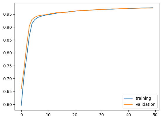
plt.plot(history.history["accuracy"],label='training')
plt.plot(history.history["val_accuracy"],label='validation')
plt.legend()

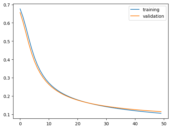
plt.plot(history.history["loss"],label='training')
plt.plot(history.history["val_loss"],label='validation')
plt.legend()

Compared to the previous two models, model3 appears to perform the best, because its accuracy ranges between 97% and 97.31% towards the last 10 epochs. Though it’s not as high as the other two models, model3 is able to consistently score at least 97% validation accuracy. Whereas the other two models often fluctuate between 96% and 97%.

4. Model Evaluation

We will now use model3 to test my model performance on unseen data.

# load test data
test_url = "https://github.com/PhilChodrow/PIC16b/blob/master/datasets/fake_news_test.csv?raw=true"
test_data = pd.read_csv(train_url)
test_data.head()

	Unnamed: 0	title	text	fake
0	17366	Merkel: Strong result for Austria's FPO 'big c...	German Chancellor Angela Merkel said on Monday...	0
1	5634	Trump says Pence will lead voter fraud panel	WEST PALM BEACH, Fla.President Donald Trump sa...	0
2	17487	JUST IN: SUSPECTED LEAKER and “Close Confidant...	On December 5, 2017, Circa s Sara Carter warne...	1
3	12217	Thyssenkrupp has offered help to Argentina ove...	Germany s Thyssenkrupp, has offered assistance...	0
4	5535	Trump say appeals court decision on travel ban...	President Donald Trump on Thursday called the ...	0

test = make_dataset(test_data)
loss, accuracy = model3.evaluate(test)
print("Test Loss:", loss)
print("Test Accuracy:", accuracy)

225/225 ━━━━━━━━━━━━━━━━━━━━ 2s 10ms/step - accuracy: 0.9737 - loss: 0.1090
Test Loss: 0.10588612407445908
Test Accuracy: 0.9754109382629395

It appears that model3 managed to get a test accuracy of 97.5%, which is great!

5. Embedding Visualization

Let’s visualize and comment on the embedding that model3 learned.

# to display plotly plots on quarto
import plotly.io as pio
pio.renderers.default="iframe"

import numpy as np
from sklearn.decomposition import PCA
import plotly.express as px

weights = model3.get_layer('embedding').get_weights()[0]

vocab = title_vectorize_layer.get_vocabulary()

pca = PCA(n_components=2)
reduced_weights = pca.fit_transform(weights)
embedding_df = pd.DataFrame({
    'word': vocab,
    'x0': reduced_weights[:, 0],
    'x1': reduced_weights[:, 1]
})

fig = px.scatter(embedding_df,
                 x="x0",
                 y="x1",
                 hover_name="word",  # shows the word on hover
                 title="2D PCA of Word Embeddings",
                 width=800,
                 height=600)
fig.update_traces(marker=dict(size=5,
                              line=dict(width=1,
                                        color='DarkSlateGrey')),
                  selector=dict(mode='markers'))
fig.show()

In the graph above, the embedding of the words “Wednesday”, “Thursday”, “Monday”, “Tueday”, and “Friday” appear to be clustered together but not inside the central cluster. Moreover, their x1 values appear to be close to 0. Whereas their x0 values appear to range between -16 and -19. Since they are clustered outside of the central cluster, this means that these words likely do not help one differentiate between fake and real news.

Moreover, the fact that they are clustered together also makes sense, because all of them are days of the week.